Disturbances

Every system folder carries a sim_dist.txt that schedules its events: faults and their clearing, line openings, load steps and setpoint steps. This notebook applies the shipped load step of the Kundur two-area system and reads the classic inter-area response from the trajectories.

The system: twelve buses, four subtransient machines with exciters (G1 and G2 in area 1, G3 and G4 in area 2) and three ZIP loads. The event is a +50 MW load step at bus B9 at t = 1 s:

import matplotlib.pyplot as plt

import hermess

print((hermess.SYSTEMS_DIR / "kundur" / "sim_dist.txt").read_text())

# This file contains all simulation disturbances.

#Disturbance, time = 7.0, type = "FAULT_LINE", bus_i = "5", bus_j = "8", y = 30
#Disturbance, time = 7.04, type = "OPEN_LINE", bus_i = "5", bus_j = "8"
#Disturbance, time = 7.0, type = "FAULT_BUS", bus = "5", y = 80
#Disturbance, time = 7.04, type = "CLEAR_FAULT_BUS", bus = "5"
Disturbance, time = 1.0, type = "LOAD", bus ="B9", p_delta = 50, q_delta = 0

The commented lines document the other event types the parser accepts. Run the system with the quasi-static network, which is the natural setting for an electromechanical study:

dae = hermess.simulate("kundur", T_end=15.0, ts=5e-3, line_dyn=False)
res = hermess.extract_results(dae)

Simulation: 100%|██████████| 100.0/100% [00:00<00:00]

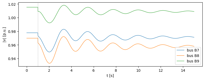
The voltages near the stepped load dip and recover as the exciters respond:

fig, ax = plt.subplots(figsize=(8, 3.2))
for bus in ["B7", "B8", "B9"]:
    ax.plot(res.t, res.voltage_magnitude(bus), lw=0.9, label=f"bus {bus}")
ax.axvline(1.0, color="0.6", ls=":", lw=1)
ax.set_xlabel("t [s]")
ax.set_ylabel("|v| [p.u.]")
ax.legend()
fig.tight_layout()

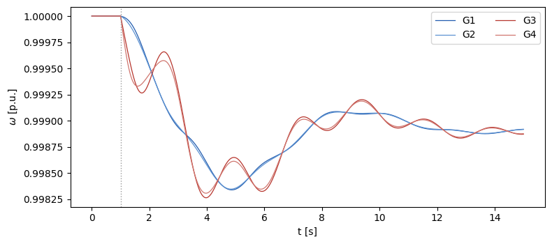
The rotor speeds show why this system is the textbook case for inter-area oscillations: G1 and G2 swing together against G3 and G4, at a frequency well below the local machine modes, and the oscillation decays slowly:

colors = {"G1": "#215CAF", "G2": "#5C92D2", "G3": "#B7352D", "G4": "#D0766F"}
fig, ax = plt.subplots(figsize=(8, 3.6))
for dev in res.devices:
    ax.plot(res.t, dev.states["omega"], lw=0.9,
            color=colors[dev.unit], label=dev.unit)
ax.axvline(1.0, color="0.6", ls=":", lw=1)
ax.set_xlabel("t [s]")
ax.set_ylabel(r"$\omega$ [p.u.]")
ax.legend(ncol=2)
fig.tight_layout()

To design an event sequence of your own, copy a system folder, edit its sim_dist.txt, and point the simulator at the parent directory:

dae = hermess.simulate("my_case", system_root="~/my_systems", T_end=10.0)

The disturbances page of the user guide documents every event type and its fields.