One system, RMS and EMT

In HERMESS the network model is a per-run switch. With line_dyn=False the network is quasi-static: the current balance is algebraic, which is the phasor (RMS) setting of classic stability programs. With line_dyn=True every line current and bus voltage becomes a differential state, so the network carries its own electromagnetic transients.

For a converter the choice extends to its output filter. The dynamic LCL filter carries the fast filter states that only make sense on a dynamic network; LCL_static is its quasi-static counterpart. The filter is a strategy selected in the system file, so the comparison also demonstrates the workflow for a modified system: copy the shipped 3bus folder (a Sauer-Pai machine, a grid-forming converter and a ZIP load, with the line between buses 3 and 1 opening at t = 3 s), select the quasi-static filter in the copy, and point simulate at it with system_root:

import shutil
import tempfile
from pathlib import Path

import matplotlib.pyplot as plt

import hermess

root = Path(tempfile.mkdtemp())
shutil.copytree(hermess.SYSTEMS_DIR / "3bus", root / "3bus_static")
par = root / "3bus_static" / "sim_param.txt"
par.write_text(par.read_text().replace(
    'GridForming, ', 'GridForming, filter = "LCL_static", '))

2572

Run the copy on the quasi-static network and the shipped original on the dynamic one:

rms = hermess.extract_results(hermess.simulate(
    "3bus_static", system_root=root, T_end=6.0, ts=1e-3, line_dyn=False))
emt = hermess.extract_results(hermess.simulate(
    "3bus", T_end=6.0, ts=1e-4, line_dyn=True))
print(f"quasi-static: {len(rms.t)} steps, dynamic network: {len(emt.t)} steps")

Simulation: 100%|██████████| 100.0/100% [00:00<00:00]
Simulation: 100%|██████████| 100.0/100% [00:01<00:00]

quasi-static: 6000 steps, dynamic network: 60000 steps

The model size follows the network choice. With the quasi-static filter the six filter states (Vfd_ext … itq_ext) turn algebraic and only the control states remain:

for name, res in (("quasi-static", rms), ("dynamic", emt)):
    gfm = next(d for d in res.devices if d.unit == "GFMI2")
    print(f"{name:>12}: {len(gfm.states):2d} converter states "
          f"({', '.join(sorted(gfm.states))})")

quasi-static:  7 converter states (Pc_tilde, Qc_tilde, delta_c, gamma_d, gamma_q, xi_d, xi_q)
     dynamic: 13 converter states (Pc_tilde, Qc_tilde, Vfd_ext, Vfq_ext, delta_c, gamma_d, gamma_q, ifd_ext, ifq_ext, itd_ext, itq_ext, xi_d, xi_q)

At the converter bus the two runs agree on the envelope over the full window:

fig, ax = plt.subplots(figsize=(8, 3.2))
ax.plot(emt.t, emt.voltage_magnitude("3"), color="#215CAF", lw=0.8,
        label="dynamic network, LCL")
ax.plot(rms.t, rms.voltage_magnitude("3"), color="#B7352D", ls="--", lw=1.2,
        label="quasi-static network, LCL_static")
ax.axvline(3.0, color="0.6", ls=":", lw=1)
ax.set_xlabel("t [s]")
ax.set_ylabel(r"$|v_3|$ [p.u.]")
ax.legend()
fig.tight_layout()

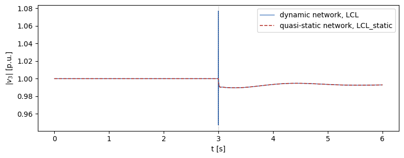
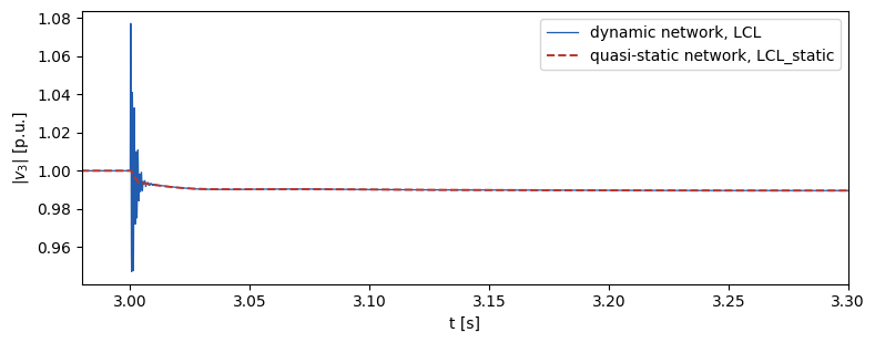
The difference lives in the milliseconds after the event. The quasi-static run jumps to the new algebraic solution; the dynamic run rings at the network and filter frequencies before settling onto the same envelope:

fig, ax = plt.subplots(figsize=(8, 3.2))
ax.plot(emt.t, emt.voltage_magnitude("3"), color="#215CAF", lw=0.9,
        label="dynamic network, LCL")
ax.plot(rms.t, rms.voltage_magnitude("3"), color="#B7352D", ls="--", lw=1.4,
        label="quasi-static network, LCL_static")
ax.set_xlim(2.98, 3.3)
ax.set_xlabel("t [s]")
ax.set_ylabel(r"$|v_3|$ [p.u.]")
ax.legend()
fig.tight_layout()

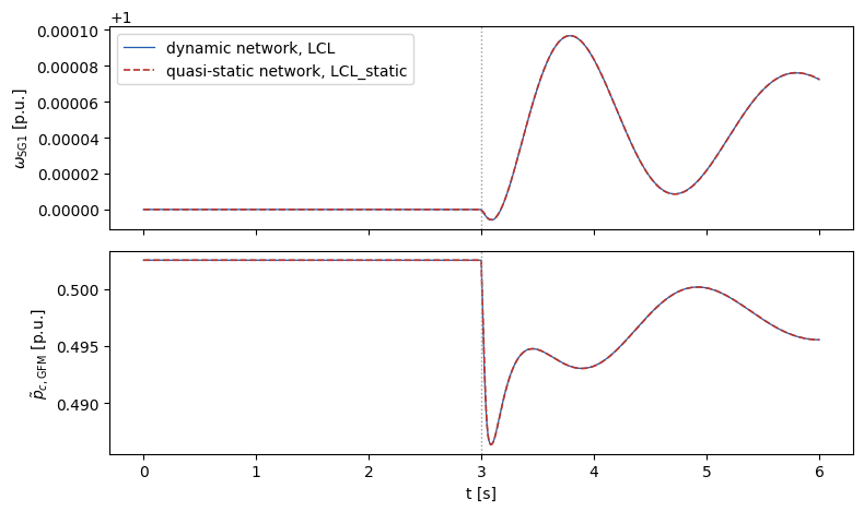
The electromechanical story is identical in both settings: the machine speed and the converter’s filtered active power overlay to within microseconds-per-unit. That is the point of the hybrid formulation. The quasi-static model answers stability questions at a fraction of the cost (6000 versus 60000 steps here), and the dynamic model is there when the fast dynamics themselves are the question, converter controls interacting with the network above all.

sg_rms = next(d for d in rms.devices if d.unit == "SG1")
sg_emt = next(d for d in emt.devices if d.unit == "SG1")
gfm_rms = next(d for d in rms.devices if d.unit == "GFMI2")
gfm_emt = next(d for d in emt.devices if d.unit == "GFMI2")

fig, axes = plt.subplots(2, 1, figsize=(8, 4.8), sharex=True)
axes[0].plot(emt.t, sg_emt.states["omega"], color="#215CAF", lw=0.9,
             label="dynamic network, LCL")
axes[0].plot(rms.t, sg_rms.states["omega"], color="#B7352D", ls="--", lw=1.2,
             label="quasi-static network, LCL_static")
axes[0].set_ylabel(r"$\omega_{\mathrm{SG1}}$ [p.u.]")
axes[0].legend()
axes[1].plot(emt.t, gfm_emt.states["Pc_tilde"], color="#215CAF", lw=0.9)
axes[1].plot(rms.t, gfm_rms.states["Pc_tilde"], color="#B7352D", ls="--",
             lw=1.2)
axes[1].set_ylabel(r"$\tilde p_{c,\mathrm{GFM}}$ [p.u.]")
axes[1].set_xlabel("t [s]")
for ax in axes:
    ax.axvline(3.0, color="0.6", ls=":", lw=1)
fig.tight_layout()