Converter control strategies

The blocks plugged onto a converter, selected by keyword on the converter line, for example filter = "LCL_static", angle = "Droop", pll = "SRF_PLL". How the five axes fit together is shown in Converters.

Output filters (filter = ...)

filter =	Class	Description
"LCL"	LCL	Dynamic LCL output filter (the framework default): series \(r_f\)-\(l_f\) converter branch, shunt capacitor \(c_f\), series \(r_t\)-\(l_t\) grid branch, with all six electrical quantities as differential states (cf. https://doi.org/10.1109/TPWRS.2021.3061434).
"LCL_static"	LCL_static	Quasi-static LCL filter: same topology and parameters as LCL, but the six filter quantities are device-private algebraic variables instead of differential states (the singular-perturbation reduction zeroing the fast LCL dynamics, \(d/dt \to 0\)).

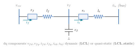
The LCL output filter between the switching voltage and the bus.

class hermess.devices.inverter_filter.LCL

Dynamic LCL output filter (the framework default): series \(r_f\)-\(l_f\) converter branch, shunt capacitor \(c_f\), series \(r_t\)-\(l_t\) grid branch, with all six electrical quantities as differential states (cf. https://doi.org/10.1109/TPWRS.2021.3061434).

Selected on a converter line with filter = "LCL".

Model. All quantities are in the network (external) dq frame, whose axes coincide with the real/imaginary axes of the network phasors; \(v_{n,re}, v_{n,im}\) are the bus-voltage components, \(\omega_b = 2 \pi f_n\) the base speed, and \(\omega_{ref}\) the per-bus reference-frame frequency. The switching voltage \(v_{swd}, v_{swq}\) comes from the inner controller through the host. This class writes all six ODEs; the host contributes the network current injection built from \(i_{td}, i_{tq}\) and the Park transforms the control ladder reads.

Capacitor voltage:

\[\begin{split}\dot{v}_{fd} &= \frac{\omega_b}{c_f} \left( i_{fd} - i_{td} \right) + \omega_{ref} \, \omega_b \, v_{fq} \\ \dot{v}_{fq} &= \frac{\omega_b}{c_f} \left( i_{fq} - i_{tq} \right) - \omega_{ref} \, \omega_b \, v_{fd}\end{split}\]

Converter-side filter current:

\[\begin{split}\dot{i}_{fd} &= \frac{\omega_b}{l_f} \left( v_{swd} - v_{fd} \right) - \frac{\omega_b r_f}{l_f} i_{fd} + \omega_{ref} \, \omega_b \, i_{fq} \\ \dot{i}_{fq} &= \frac{\omega_b}{l_f} \left( v_{swq} - v_{fq} \right) - \frac{\omega_b r_f}{l_f} i_{fq} - \omega_{ref} \, \omega_b \, i_{fd}\end{split}\]

Terminal (grid-side) current:

\[\begin{split}\dot{i}_{td} &= \frac{\omega_b}{l_t} \left( v_{fd} - v_{n,re} \right) - \frac{\omega_b r_t}{l_t} i_{td} + \omega_{ref} \, \omega_b \, i_{tq} \\ \dot{i}_{tq} &= \frac{\omega_b}{l_t} \left( v_{fq} - v_{n,im} \right) - \frac{\omega_b r_t}{l_t} i_{tq} - \omega_{ref} \, \omega_b \, i_{td}\end{split}\]

All parameters are per unit on the device base; at nominal frequency the per-unit inductances and capacitance equal the corresponding reactances and susceptance.

Symbols.

Code	Symbol	Meaning	Default
Rf	\(r_f\)	converter-branch (filter) resistance [p.u.]	1e-4
Lf	\(l_f\)	converter-branch (filter) inductance [p.u.]	0.08
Cf	\(c_f\)	shunt (filter) capacitance [p.u.]	0.074
Rt	\(r_t\)	grid-branch resistance (filter to terminal) [p.u.]	0.01
Lt	\(l_t\)	grid-branch inductance (filter to terminal) [p.u.]	0.2
Vfd_ext / Vfq_ext	\(v_{fd},\ v_{fq}\)	capacitor voltage, network dq frame (states) [p.u.]
ifd_ext / ifq_ext	\(i_{fd},\ i_{fq}\)	converter-side filter current (states) [p.u.]
itd_ext / itq_ext	\(i_{td},\ i_{tq}\)	terminal current into the grid (states) [p.u.]

class hermess.devices.inverter_filter.LCL_static

Quasi-static LCL filter: same topology and parameters as LCL, but the six filter quantities are device-private algebraic variables instead of differential states (the singular-perturbation reduction zeroing the fast LCL dynamics, \(d/dt \to 0\)). Appropriate when the network itself is quasi-static (line_dyn=False); a dynamic filter on a static network is physically incoherent (the host warns but allows it).

Selected on a converter line with filter = "LCL_static".

Model. The LCL equations with the derivatives zeroed. The factor \(\omega_b\) common to every term is dropped from each constraint: it is mathematically redundant and would inflate the initialization Jacobian’s condition number.

\[\begin{split}0 &= \frac{1}{c_f} \left( i_{fd} - i_{td} \right) + \omega_{ref} \, v_{fq} \\ 0 &= \frac{1}{c_f} \left( i_{fq} - i_{tq} \right) - \omega_{ref} \, v_{fd} \\ 0 &= \frac{1}{l_f} \left( v_{swd} - v_{fd} \right) - \frac{r_f}{l_f} i_{fd} + \omega_{ref} \, i_{fq} \\ 0 &= \frac{1}{l_f} \left( v_{swq} - v_{fq} \right) - \frac{r_f}{l_f} i_{fq} - \omega_{ref} \, i_{fd} \\ 0 &= \frac{1}{l_t} \left( v_{fd} - v_{n,re} \right) - \frac{r_t}{l_t} i_{td} + \omega_{ref} \, i_{tq} \\ 0 &= \frac{1}{l_t} \left( v_{fq} - v_{n,im} \right) - \frac{r_t}{l_t} i_{tq} - \omega_{ref} \, i_{td}\end{split}\]

Symbols. As for LCL (parameters Rf, Lf, Cf, Rt, Lt are inherited unchanged); the six quantities Vfd_ext / Vfq_ext, ifd_ext / ifq_ext, itd_ext / itq_ext are private algebraics here instead of states.

Angle sources (angle = ...)

The angle source fixes how the converter synchronizes. Droop is the grid-forming active-power droop, and PLL adds the same droop on the PLL frequency for a grid-supporting unit. VSM is a virtual-synchronous-machine swing with virtual inertia, damped against the PLL frequency. PLLPowerPI is the grid-following choice, which aliases the converter frame to the PLL frame and turns the active-power error into the d-axis current command.

angle =	Class	Description
"Droop"	DroopAngle	Grid-forming droop angle source: the converter sets its own frequency from the active-power droop off the nominal frequency.
"PLL"	PLLAngle	Grid-following angle source: the converter frequency rides on the PLL’s synchronizing frequency plus the active-power droop.
"PLLPowerPI"	PLLPowerPI	PLL-synchronized active-power PI: the converter frame IS the PLL frame (no angle state of its own), and a PI on the filtered active power produces the d-axis current command consumed by a current-mode inner control (the PSID ActivePowerPI grid-following outer; pairs with voltage = "QPowerPI" and inner = "CurrentPI").
"VSM"	VSMAngle	Virtual-synchronous-machine angle source: the converter frequency is a state driven by the unfiltered power imbalance through a virtual inertia, damped against the PLL frequency and the nominal frequency (the D’Arco/PSID VirtualInertia outer control; requires a PLL strategy for the damping term).

class hermess.devices.inverter_angle.DroopAngle

Grid-forming droop angle source: the converter sets its own frequency from the active-power droop off the nominal frequency.

Selected on a converter line with angle = "Droop".

Model.

\[\begin{split}\omega_c &= \omega_{net} + R_c^{p} \left( p_c^{*} - \tilde{p}_c \right) \\ \dot{\delta}_c &= \omega_b \left( \omega_c - \omega_{ref} \right)\end{split}\]

The filtered active power obeys the measurement filter \(\dot{\tilde{p}}_c = \omega_f ( p_c - \tilde{p}_c )\), written by the host converter (\(p_c\) comes from the shared Park-transform loop in Inverter.fgcall). \(\omega_{ref}\) is the reference frequency selected by omega_mode and \(\omega_{net}\) the nominal network frequency (1 p.u.). The converter frequency is exposed as host.omega_c (read by the center-of-inertia / single reference-frame machinery in system.py).

Symbols.

Code	Symbol	Meaning	Default
Kp	\(R_c^{p}\)	P-f droop coefficient	0.02
Pc_tilde	\(\tilde{p}_c\)	filtered active power (state) [p.u.]
delta_c	\(\delta_c\)	converter-frame angle relative to the network (state) [rad]
Pref	\(p_c^{*}\)	active-power setpoint (set to \(p_c\) by the initialization)

class hermess.devices.inverter_angle.PLLAngle

Grid-following angle source: the converter frequency rides on the PLL’s synchronizing frequency plus the active-power droop. Pairs with a PLL strategy (which owns \(\omega_{pll}\) and the PLL states).

Selected on a converter line with angle = "PLL".

Model.

\[\begin{split}\omega_c &= \omega_{pll} + R_c^{p} \left( p_c^{*} - \tilde{p}_c \right) \\ \dot{\delta}_c &= \omega_b \left( \omega_c - \omega_{ref} \right)\end{split}\]

with \(\omega_{pll}\) the synchronizing frequency estimated by the PLL strategy (read host-mediated via host.pll_frequency). The filtered active power obeys \(\dot{\tilde{p}}_c = \omega_f ( p_c - \tilde{p}_c )\), written by the host converter; \(\omega_{ref}\) is the reference frequency selected by omega_mode.

Symbols.

Code	Symbol	Meaning	Default
Kp	\(R_c^{p}\)	P-f droop coefficient	0.02
Pc_tilde	\(\tilde{p}_c\)	filtered active power (state) [p.u.]
delta_c	\(\delta_c\)	converter-frame angle relative to the network (state) [rad]
Pref	\(p_c^{*}\)	active-power setpoint (set to \(p_c\) by the initialization)

class hermess.devices.inverter_angle.VSMAngle

Virtual-synchronous-machine angle source: the converter frequency is a state driven by the unfiltered power imbalance through a virtual inertia, damped against the PLL frequency and the nominal frequency (the D’Arco/PSID VirtualInertia outer control; requires a PLL strategy for the damping term).

Selected on a converter line with angle = "VSM".

Model.

\[\begin{split}T_a \, \dot{\omega}_{vsm} &= p_c^{*} - p_c - K_d \left( \omega_{vsm} - \omega_{pll} \right) - K_w \left( \omega_{vsm} - \omega_{net} \right) \\ \dot{\delta}_c &= \omega_b \left( \omega_{vsm} - \omega_{ref} \right)\end{split}\]

with \(p_c\) the UNFILTERED converter power (host Park loop; the VSM carries its own inertia instead of a measurement filter) and \(\omega_{pll}\) the PLL estimate via host.pll_frequency. The converter frequency exposed to the inner ladder and the reference-frame machinery is \(\omega_{vsm}\) itself.

Symbols.

Code	Symbol	Meaning	Default
Ta	\(T_a\)	virtual (VSM) inertia constant [s]	2
Kd	\(K_d\)	VSM damping gain (against the PLL frequency)	400
Kw	\(K_w\)	frequency droop gain (against nominal)	20
omega_vsm	\(\omega_{vsm}\)	virtual rotor speed (state) [p.u.]
delta_c	\(\delta_c\)	converter-frame angle relative to the network (state) [rad]
Pref	\(p_c^{*}\)	active-power setpoint (set to \(p_c\) by the initialization)

class hermess.devices.inverter_angle.PLLPowerPI

PLL-synchronized active-power PI: the converter frame IS the PLL frame (no angle state of its own), and a PI on the filtered active power produces the d-axis current command consumed by a current-mode inner control (the PSID ActivePowerPI grid-following outer; pairs with voltage = "QPowerPI" and inner = "CurrentPI").

Selected on a converter line with angle = "PLLPowerPI".

Model. The frame angle is a device-private algebraic aliased to the PLL angle, and the current command is

\[\begin{split}0 &= -\delta_c + \delta_{pll}, \qquad \omega_c = \omega_{pll} \\ i_{d}^{cmd} &= K_p^{p} \left( p_c^{*} - \tilde{p}_c \right) + K_i^{p} \, \sigma_p, \qquad \dot{\sigma}_p = p_c^{*} - \tilde{p}_c\end{split}\]

with \(\tilde{p}_c\) the host’s filtered active power (corner omega_f). Published on host.Idc_cmd (read by the inner control via host.current_command).

Symbols.

Code	Symbol	Meaning	Default
Kpp	\(K_p^{p}\)	active-power PI proportional gain	2
Pc_tilde	\(\\tilde{p}_c\)	filtered active power (state) [p.u.]
Kip	\(K_i^{p}\)	active-power PI integral gain	30
sigma_p	\(\sigma_p\)	active-power PI integrator (state) [p.u.]
delta_c	\(\delta_c\)	converter-frame angle (private algebraic, = \(\delta_{pll}\)) [rad]
Pref	\(p_c^{*}\)	active-power setpoint (set to \(p_c\) by the initialization)

Voltage control (voltage = ...)

QVDroop turns the reactive-power error into the voltage-magnitude command of the voltage-mode cascade. QPowerPI replaces it in the current-injecting chain and produces the q-axis current command instead.

voltage =	Class	Description
"QPowerPI"	QPowerPI	Reactive-power PI: a PI on the filtered reactive power produces the q-axis current command consumed by a current-mode inner control (the PSID ReactivePowerPI grid-following outer; pairs with angle = "PLLPowerPI" and inner = "CurrentPI").
"QVDroop"	QVDroop	Reactive-power / voltage droop: the voltage-magnitude command follows the reactive-power deviation from its setpoint.

class hermess.devices.inverter_voltage.QVDroop

Reactive-power / voltage droop: the voltage-magnitude command follows the reactive-power deviation from its setpoint.

Selected on a converter line with voltage = "QVDroop".

Model. The command is algebraic (published on host.Vcd, read by the inner control ladder):

\[v_{cd} = v_c^{*} + R_c^{q} \left( q_c^{*} - \tilde{q}_c \right)\]

The filtered reactive power obeys the measurement filter \(\dot{\tilde{q}}_c = \omega_f ( q_c - \tilde{q}_c )\), written by the host converter (\(q_c\) comes from the shared Park-transform loop in Inverter.fgcall). The droop is static, so at initialization \(q_c^{*}\) and \(v_c^{*}\) form a one-parameter gauge fixed by the convention \(q_c^{*} = q_c\) (zeroing the droop term), which gives \(v_c^{*} = v_{cd}\).

Symbols.

Code	Symbol	Meaning	Default
Kq	\(R_c^{q}\)	Q-V droop coefficient	0.1
Qc_tilde	\(\tilde{q}_c\)	filtered reactive power (state) [p.u.]
Qref	\(q_c^{*}\)	reactive-power setpoint (set to \(q_c\) by the initialization)
Vref	\(v_c^{*}\)	voltage setpoint (set to \(v_{cd}\) by the initialization)

class hermess.devices.inverter_voltage.QPowerPI

Reactive-power PI: a PI on the filtered reactive power produces the q-axis current command consumed by a current-mode inner control (the PSID ReactivePowerPI grid-following outer; pairs with angle = "PLLPowerPI" and inner = "CurrentPI").

Selected on a converter line with voltage = "QPowerPI".

Model.

\[i_{q}^{cmd} &= -\left[ K_p^{q} \left( q_c^{*} - \tilde{q}_c \right) + K_i^{q} \, \sigma_q \right], \qquad \dot{\sigma}_q = q_c^{*} - \tilde{q}_c\]

with \(\tilde{q}_c\) the host’s filtered reactive power. The q-axis gain is negative because the PLL drives the frame’s q-voltage to zero, so \(q_c \approx -v_d i_q\). Published on host.Iqc_cmd (read by the inner control via host.current_command); no voltage-magnitude command is produced.

Symbols.

Code	Symbol	Meaning	Default
Kpq	\(K_p^{q}\)	reactive-power PI proportional gain	2
Qc_tilde	\(\\tilde{q}_c\)	filtered reactive power (state) [p.u.]
Kiq	\(K_i^{q}\)	reactive-power PI integral gain	30
sigma_q	\(\sigma_q\)	reactive-power PI integrator (state) [p.u.]
Qref	\(q_c^{*}\)	reactive-power setpoint (set to \(q_c\) by the initialization)

Inner control (inner = ...)

Cascaded closes the voltage and current loops of the voltage-mode cascade, and CascadedDamped adds capacitor-voltage active damping on top of it. CurrentPI is the current-mode loop of the grid-following chain, tracking the commands of the power PIs directly.

inner =	Class	Description
"Cascaded"	Cascaded	Cascaded voltage and current PI control with virtual impedance (the standard two-loop vector control of a voltage-forming converter; cf. https://doi.org/10.1109/TPWRS.2021.3061434).
"CascadedDamped"	CascadedDamped	Cascaded with capacitor-voltage active damping: the filter voltage is high-pass filtered (gain \(K_{ad}\), corner \(\omega_{ad}\)) and subtracted from the switching-voltage reference, damping the LC resonance (the D’Arco VoltageModeControl with its active damping enabled; Cascaded is the \(K_{ad} = 0\) special case without the two filter states).
"CurrentPI"	CurrentPI	Current-mode inner control: a single PI tracks the converter-side filter current against the commands published by the power PI outers, with inductor decoupling and capacitor-voltage feed-forward (the PSID CurrentModeControl; pairs with angle = "PLLPowerPI" and voltage = "QPowerPI").

class hermess.devices.inverter_inner.Cascaded

Cascaded voltage and current PI control with virtual impedance (the standard two-loop vector control of a voltage-forming converter; cf. https://doi.org/10.1109/TPWRS.2021.3061434).

Selected on a converter line with inner = "Cascaded".

Model. All quantities are in the converter (internal) dq frame, the host’s Park transform of the network-frame filter states by the frame angle \(\delta_c\); \(\omega_c\) is the converter frequency from the angle source and \(V_{cd}\) the d-axis voltage command from the outer voltage controller (the q-command is implicitly zero). The voltage references include the virtual-impedance drop over the terminal current:

\[\begin{split}v_{fd}^{*} &= V_{cd} - R_v \, i_{td} + \omega_c L_v \, i_{tq} \\ v_{fq}^{*} &= - R_v \, i_{tq} - \omega_c L_v \, i_{td}\end{split}\]

The voltage PI (with capacitor decoupling and terminal-current feed-forward) produces the filter-current references:

\[\begin{split}i_{fd}^{*} &= K_p^v \left( v_{fd}^{*} - v_{fd} \right) + K_i^v \, \xi_d - \omega_c c_f \, v_{fq} + K_{ff}^v \, i_{td} \\ i_{fq}^{*} &= K_p^v \left( v_{fq}^{*} - v_{fq} \right) + K_i^v \, \xi_q + \omega_c c_f \, v_{fd} + K_{ff}^v \, i_{tq}\end{split}\]

and the current PI (with inductor decoupling and capacitor-voltage feed-forward) the switching voltage:

\[\begin{split}v_{swd} &= K_p^c \left( i_{fd}^{*} - i_{fd} \right) + K_i^c \, \gamma_d - \omega_c l_f \, i_{fq} + K_{ff}^c \, v_{fd} \\ v_{swq} &= K_p^c \left( i_{fq}^{*} - i_{fq} \right) + K_i^c \, \gamma_q + \omega_c l_f \, i_{fd} + K_{ff}^c \, v_{fq}\end{split}\]

which is rotated back to the network frame by \(\delta_c\) and published on the host (read by the filter strategy). The four PI integrators are the strategy’s differential states:

\[\dot{\xi}_d = v_{fd}^{*} - v_{fd}, \quad \dot{\xi}_q = v_{fq}^{*} - v_{fq}, \quad \dot{\gamma}_d = i_{fd}^{*} - i_{fd}, \quad \dot{\gamma}_q = i_{fq}^{*} - i_{fq}\]

The decoupling terms read the filter parameters \(c_f\) and \(l_f\) from the host, so this controller presupposes a shunt-capacitor (LC/LCL) plant; the current references pass through the host accessor host.current_ref, the interception seam for a future current limiter.

Symbols.

Code	Symbol	Meaning	Default
Kpv	\(K_p^v\)	voltage-loop proportional gain	0.59
Kiv	\(K_i^v\)	voltage-loop integral gain	736
Kffv	\(K_{ff}^v\)	voltage-loop (terminal-current) feed-forward gain	0
Kpc	\(K_p^c\)	current-loop proportional gain	1.27
Kic	\(K_i^c\)	current-loop integral gain	14.3
Kffc	\(K_{ff}^c\)	current-loop (capacitor-voltage) feed-forward gain	0
Rv	\(R_v\)	virtual resistance [p.u.]	0
Lv	\(L_v\)	virtual inductance [p.u.]	0.2
xi_d / xi_q	\(\xi_d,\ \xi_q\)	voltage-loop integrator states [p.u.]
gamma_d / gamma_q	\(\gamma_d,\ \gamma_q\)	current-loop integrator states [p.u.]

class hermess.devices.inverter_inner.CascadedDamped

Cascaded with capacitor-voltage active damping: the filter voltage is high-pass filtered (gain \(K_{ad}\), corner \(\omega_{ad}\)) and subtracted from the switching-voltage reference, damping the LC resonance (the D’Arco VoltageModeControl with its active damping enabled; Cascaded is the \(K_{ad} = 0\) special case without the two filter states).

Selected on a converter line with inner = "CascadedDamped".

Model. As Cascaded, with the switching-voltage references extended by the damping term and the two low-pass states:

\[\begin{split}v_{swd} &\mathrel{{-}{=}} K_{ad} \left( v_{fd} - \phi_d \right), \qquad v_{swq} \mathrel{{-}{=}} K_{ad} \left( v_{fq} - \phi_q \right) \\ \dot{\phi}_d &= \omega_{ad} \left( v_{fd} - \phi_d \right), \qquad \dot{\phi}_q = \omega_{ad} \left( v_{fq} - \phi_q \right)\end{split}\]

Symbols. As Cascaded, plus:

Code	Symbol	Meaning	Default
Kad	\(K_{ad}\)	active damping gain	0.2
omega_ad	\(\omega_{ad}\)	active damping low-pass corner frequency [rad/s]	50
phi_d / phi_q	\(\phi_d,\ \phi_q\)	active damping low-pass states [p.u.]

class hermess.devices.inverter_inner.CurrentPI

Current-mode inner control: a single PI tracks the converter-side filter current against the commands published by the power PI outers, with inductor decoupling and capacitor-voltage feed-forward (the PSID CurrentModeControl; pairs with angle = "PLLPowerPI" and voltage = "QPowerPI").

Selected on a converter line with inner = "CurrentPI".

Model. In the converter frame (the PLL frame):

\[\begin{split}v_{swd} &= K_p^c \left( i_{d}^{cmd} - i_{fd} \right) + K_i^c \, \gamma_d - \omega_c l_f \, i_{fq} + K_{ff}^c \, v_{fd} \\ v_{swq} &= K_p^c \left( i_{q}^{cmd} - i_{fq} \right) + K_i^c \, \gamma_q + \omega_c l_f \, i_{fd} + K_{ff}^c \, v_{fq} \\ \dot{\gamma}_d &= i_{d}^{cmd} - i_{fd}, \qquad \dot{\gamma}_q = i_{q}^{cmd} - i_{fq}\end{split}\]

The commands come host-mediated from host.current_command; the voltage feed-forward is enabled by default (\(K_{ff}^c = 1\)), as in the reference model.

Symbols.

Code	Symbol	Meaning	Default
Kpc	\(K_p^c\)	current-loop proportional gain	0.37
Kic	\(K_i^c\)	current-loop integral gain	0.7
Kffc	\(K_{ff}^c\)	capacitor-voltage feed-forward gain	1
gamma_d / gamma_q	\(\gamma_d,\ \gamma_q\)	current-loop integrator states [p.u.]

Phase-locked loops (pll = ...)

pll =	Class	Description
"Kaura"	KauraPLL	Kaura-Blasko PLL: low-pass filters on both dq components of the measured filter voltage and a phase detector on their angle (Kaura and Blasko 1997; the PSID/PSCAD virtual-synchronous-machine reference uses it).
"ReducedPLL"	ReducedPLL	Reduced-order PLL: the SRF_PLL with a first-order low-pass filter on the measured q-axis voltage (the reduced-order PLL of the PSID grid-following reference model).
"SRF_PLL"	SRF_PLL	Synchronous-reference-frame PLL: locks the PLL frame to the filter voltage by driving its q-axis component to zero through a PI loop.

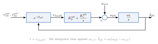
Synchronous-reference-frame PLL: the q-component of the filter voltage is driven to zero, locking \(\delta_{pll}\) to the filter-voltage phasor.

SRF_PLL is the synchronous-reference-frame loop of the figure. ReducedPLL low-pass filters the measured q-voltage before the loop, and Kaura filters both axes and acts on the phase angle of the filtered phasor.

class hermess.devices.inverter_pll.SRF_PLL

Synchronous-reference-frame PLL: locks the PLL frame to the filter voltage by driving its q-axis component to zero through a PI loop.

Selected on a converter line with pll = "SRF_PLL".

Model. The filter voltage is rotated into the PLL frame,

\[v_{fq,pll} = -v_{fd}^{ext} \sin\delta_{pll} + v_{fq}^{ext} \cos\delta_{pll},\]

and the PI loop drives it to zero:

\[\begin{split}\omega_{pll} &= \omega_{net} + K_p^{pll} \, v_{fq,pll} + K_i^{pll} \, \epsilon \\ \dot{\epsilon} &= v_{fq,pll} \\ \dot{\delta}_{pll} &= \omega_b \left( \omega_{pll} - \omega_{ref} \right)\end{split}\]

\(\omega_{pll}\) is published on host.omega_pll (an algebraic expression, not a registered variable) and read by the angle source via host.pll_frequency(dae). At steady state the PLL is locked: \(v_{fq,pll} = 0\), \(\epsilon = 0\), and \(\delta_{pll}\) is the filter-voltage angle.

Symbols.

Code	Symbol	Meaning	Default
Kpll_p	\(K_p^{pll}\)	PLL proportional gain	0.5
Kpll_i	\(K_i^{pll}\)	PLL integral gain	4.69
epsilon	\(\epsilon\)	PLL integrator state [p.u.]
delta_pll	\(\delta_{pll}\)	PLL-frame angle relative to the network (state) [rad]

class hermess.devices.inverter_pll.ReducedPLL

Reduced-order PLL: the SRF_PLL with a first-order low-pass filter on the measured q-axis voltage (the reduced-order PLL of the PSID grid-following reference model).

Selected on a converter line with pll = "ReducedPLL".

Model. The filter voltage is rotated into the PLL frame as in SRF_PLL; the PI loop acts on the low-pass-filtered q-component:

\[\begin{split}\dot{v}_{q,lp} &= \omega_{lp} \left( v_{fq,pll} - v_{q,lp} \right) \\ \omega_{pll} &= \omega_{net} + K_p^{pll} \, v_{q,lp} + K_i^{pll} \, \epsilon \\ \dot{\epsilon} &= v_{q,lp} \\ \dot{\delta}_{pll} &= \omega_b \left( \omega_{pll} - \omega_{ref} \right)\end{split}\]

In the limit \(\omega_{lp} \to \infty\) this is exactly the SRF_PLL.

Symbols. As SRF_PLL, plus:

Code	Symbol	Meaning	Default
omega_lp	\(\omega_{lp}\)	measurement low-pass corner frequency [rad/s]	414.69
vq_lp	\(v_{q,lp}\)	filtered PLL q-axis voltage (state) [p.u.]

class hermess.devices.inverter_pll.KauraPLL

Kaura-Blasko PLL: low-pass filters on both dq components of the measured filter voltage and a phase detector on their angle (Kaura and Blasko 1997; the PSID/PSCAD virtual-synchronous-machine reference uses it).

Selected on a converter line with pll = "Kaura".

Model. The filter voltage is rotated into the PLL frame and low-pass filtered on both axes; the PI loop acts on the phase error \(\operatorname{atan2}(v_{q,lp}, v_{d,lp})\):

\[\begin{split}\dot{v}_{d,lp} &= \omega_{lp} \left( v_{fd,pll} - v_{d,lp} \right) \\ \dot{v}_{q,lp} &= \omega_{lp} \left( v_{fq,pll} - v_{q,lp} \right) \\ \omega_{pll} &= \omega_{net} + K_p^{pll} \operatorname{atan2}(v_{q,lp}, v_{d,lp}) + K_i^{pll} \, \epsilon \\ \dot{\epsilon} &= \operatorname{atan2}(v_{q,lp}, v_{d,lp}) \\ \dot{\delta}_{pll} &= \omega_b \left( \omega_{pll} - \omega_{ref} \right)\end{split}\]

Near the lock (\(v_{q,lp} \approx 0\), \(v_{d,lp} \approx |v_f|\)) this linearizes to the magnitude-normalized SRF_PLL.

Symbols.

Code	Symbol	Meaning	Default
Kpll_p	\(K_p^{pll}\)	PLL proportional gain	0.084
Kpll_i	\(K_i^{pll}\)	PLL integral gain	4.69
omega_lp	\(\omega_{lp}\)	measurement low-pass corner frequency [rad/s]	500
vd_lp / vq_lp	\(v_{d,lp},\ v_{q,lp}\)	filtered PLL-frame voltages (states) [p.u.]
epsilon	\(\epsilon\)	PLL integrator state [p.u.]
delta_pll	\(\delta_{pll}\)	PLL-frame angle relative to the network (state) [rad]