Static Models

Static models carry no internal states: they contribute only to the algebraic network equations. They are declared in the system file (hermess/systems/<case>/sim_param.txt) by class name, and their classes live in hermess/devices/static.py, except the transmission line, which is part of hermess/devices/device.py.

All loads are initialized by the power flow: the powers given in the system file are replaced by the values that make the operating point a steady state at t = 0 s. See System files for the file format.

Transmission line

Branches are declared with Line. Parameters are in per unit on the system base, so transformers are represented by the off-nominal tap ratio trafo of the branch rather than by a separate model.

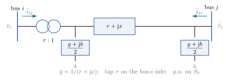
The quasi-static PI model with the off-nominal tap \(\tau\) on the bus_i side. With line_dyn=True the series branch additionally carries the electromagnetic current dynamics.

class hermess.devices.device.Line

Transmission line or transformer branch (PI model with off-nominal tap).

Selected in a system file by the class name in the first column, e.g. Line, bus_i = "1", bus_j = "2", r = 0.01, x = 0.08, g = 0.001, b = 0.03, trafo = 1. All values are per unit on the system base, so a transformer is represented by the off-nominal tap ratio \(\tau\) (trafo) of its branch rather than by a separate model.

Quasi-static model (line_dyn = False). The branch is a PI section: series impedance \(z = r + jx\) with series admittance \(\bar{y}_s = 1/z\), total shunt \(g + jb\) split half per end, and the tap on the bus_i (from) side. The class only carries the parameters; hermess.system.Grid.build_y_sym assembles the bus admittance matrix from them, with \(z^{-1} = 1/(r^2 + x^2)\) and entries (real, imaginary):

\[\begin{split}Y_{ij} = Y_{ji} &: \Bigl( -\frac{r z^{-1}}{\tau}, \; -\frac{x z^{-1}}{\tau} \Bigr) \\ Y_{ii} &: \Bigl( \frac{g/2 + r z^{-1}}{\tau^2}, \; \frac{-b/2 + x z^{-1}}{\tau^2} \Bigr) \\ Y_{jj} &: \Bigl( g/2 + r z^{-1}, \; -b/2 + x z^{-1} \Bigr)\end{split}\]

The imaginary entries are stored in the sign convention of the rectangular nodal current balance used throughout the code (the susceptance rows enter with the sign shown, i.e. a stored pair \((a, b)\) corresponds to the admittance \(a - jb\) of the standard phasor convention). During a middle-of-line fault the branch’s \(r, x, g, b\) are replaced by the equivalent PI section of the faulted T model; an opened line is removed by setting its series impedance effectively infinite.

Dynamic (electromagnetic) model (line_dyn = True). The series branch keeps its own current states \(\bar{i}_{ij} = i_{ij,re} + j \, i_{ij,im}\) (in the line’s reference frame, with the nodal voltages transformed into that frame):

\[\begin{split}\frac{d i_{ij,re}}{dt} &= \frac{\omega_b}{x} \Bigl( \frac{v_{i,re}}{\tau} - v_{j,re} - r \, i_{ij,re} \Bigr) + \omega_b \, \omega_{ref} \, i_{ij,im} \\ \frac{d i_{ij,im}}{dt} &= \frac{\omega_b}{x} \Bigl( \frac{v_{i,im}}{\tau} - v_{j,im} - r \, i_{ij,im} \Bigr) - \omega_b \, \omega_{ref} \, i_{ij,re}\end{split}\]

with \(\omega_b = 2 \pi f_n\) and \(\omega_{ref}\) the line’s reference frequency (per the configured omega_mode); here \(x\) and \(b\) act as the inductance and capacitance, being numerically equal at 1 p.u. frequency. The line switch of an opened line zeroes the derivatives, and the branch currents are accumulated into the nodal current balance transformed to the bus frame.

Symbols.

Code	Symbol	Meaning	Default
r	\(r\)	series resistance [p.u.]	0.001
x	\(x\)	series reactance [p.u.]	0.001
g	\(g\)	total shunt conductance [p.u.], split half per end	0
b	\(b\)	total shunt susceptance [p.u.], split half per end	0
trafo	\(\tau\)	off-nominal tap ratio on the bus_i side (real)	1
bus_i		name of the sending-end (from) bus
bus_j		name of the receiving-end (to) bus
i_ijr	\(i_{ij,re}\)	series current, real part (state, line_dyn only) [p.u.]
i_iji	\(i_{ij,im}\)	series current, imaginary part (state, line_dyn only) [p.u.]

ZIP load

The general static load: a combination of constant-impedance, constant-current and constant-power behavior, set by the shares z_share, i_share and p_share. This is the load model used by most of the shipped systems.

class hermess.devices.static.StaticZIP

ZIP load: constant-impedance (Z), constant-current (I) and

constant-power (P) branches in parallel, with independently chosen shares.

Selected in a system file by the class name in the first column, e.g. StaticZIP, bus = "2", z_share = 0.4, i_share = 0.3, p_share = 0.3. The shares of each branch on the active-power side must sum to one; the reactive-power side has its own shares (*_share_q) that default to the active-power values when not given.

Model. The consumed current is the sum of the three branches, with \(\theta = \operatorname{atan2}(v_{im}, v_{re})\) the voltage angle:

\[\begin{split}i_{re} &= \underbrace{\frac{p \, v_{re} + q \, v_{im}}{v_{re}^2 + v_{im}^2}}_{P} \; + \; \underbrace{g \, v_{re} - b \, v_{im}}_{Z} \; + \; \underbrace{\cos\theta \, i_d + \sin\theta \, i_q}_{I} \\ i_{im} &= \underbrace{\frac{p \, v_{im} - q \, v_{re}}{v_{re}^2 + v_{im}^2}}_{P} \; + \; \underbrace{b \, v_{re} + g \, v_{im}}_{Z} \; + \; \underbrace{\sin\theta \, i_d - \cos\theta \, i_q}_{I}\end{split}\]

The consumed powers of the branches are \(S_P = p + jq\) (constant), \(S_Z = |\bar{v}|^2 (g - jb)\) (quadratic in voltage), and \(S_I = |\bar{v}| (i_d + j i_q)\) (linear in voltage). Positive \(q\) and \(i_q\) mean reactive consumption.

Initialization. The per-bus current demanded by the power flow is decomposed into a P-only and a Q-only component,

\[\begin{split}P_0 &= v_{re} i_{re}^{0} + v_{im} i_{im}^{0}, \qquad Q_0 = v_{im} i_{re}^{0} - v_{re} i_{im}^{0}, \\ \bar{i}^{P} &= \frac{P_0}{|\bar{v}|^2} (v_{re} + j v_{im}), \qquad \bar{i}^{Q} = \frac{Q_0}{|\bar{v}|^2} (v_{im} - j v_{re}),\end{split}\]

and each branch’s setpoint pair (\((g, b)\), \((i_d, i_q)\) or \((p, q)\)) is solved by Newton iteration so that the branch consumes exactly its share-weighted portion \(s^{P} \bar{i}^{P} + s^{Q} \bar{i}^{Q}\) of that current. Shares that do not sum to one per axis are reported as a warning: the load then under- or over-delivers.

Symbols.

Code	Symbol	Meaning	Default
z_share	\(s_Z^{P}\)	impedance share of the active-power demand	1
i_share	\(s_I^{P}\)	current share of the active-power demand	0
p_share	\(s_P^{P}\)	power share of the active-power demand	0
z_share_q	\(s_Z^{Q}\)	impedance share of the reactive-power demand (default: follows z_share)	NaN
i_share_q	\(s_I^{Q}\)	current share of the reactive-power demand (default: follows i_share)	NaN
p_share_q	\(s_P^{Q}\)	power share of the reactive-power demand (default: follows p_share)	NaN
g	\(g\)	Z-branch conductance [p.u.] (set by the initialization)	1
b	\(b\)	Z-branch susceptance [p.u.] (set by the initialization)	1
id	\(i_d\)	I-branch active current [p.u.] (set by the initialization)	1
iq	\(i_q\)	I-branch reactive current [p.u.] (set by the initialization)	1
p	\(p\)	P-branch active power [p.u.] (set by the initialization)	1
q	\(q\)	P-branch reactive power [p.u.] (set by the initialization)	1
Sn	\(S_n\)	rated power [MVA]	100
Vn	\(V_n\)	rated voltage [kV]	220
fn	\(f_n\)	nominal frequency [Hz]	50

Constant-power load

A pure constant-power (PQ) load. Equivalent to a ZIP load with p_share = 1, kept as a separate class for system files that state it explicitly.

class hermess.devices.static.StaticLoadPower

Constant-power (PQ) load.

Selected in a system file by the class name in the first column, e.g. StaticLoadPower, bus = "2".

Model. The consumed current keeps \(P\) and \(Q\) constant regardless of the bus voltage:

\[\begin{split}i_{re} &= \frac{(P/S_b) \, v_{re} + (Q/S_b) \, v_{im}}{v_{re}^2 + v_{im}^2} \\ i_{im} &= \frac{(P/S_b) \, v_{im} - (Q/S_b) \, v_{re}}{v_{re}^2 + v_{im}^2}\end{split}\]

so that \(\bar{v}\,\bar{i}^{*} = (P + jQ)/S_b\) exactly. Behaviorally this is StaticZIP with p_share = 1; unlike the ZIP setpoints, \(P\) and \(Q\) are handled here in the units of the system base Sb (MW / MVAr by default).

A constant-power load has no equilibrium below the nose of the network’s PV curve; if the initialization fails at a heavily loaded bus, use StaticZIP with an impedance share instead.

Symbols.

Code	Symbol	Meaning	Default
p	\(P\)	consumed active power [MW] (set by the initialization)	0
q	\(Q\)	consumed reactive power [MVAr] (set by the initialization)	0
Sn	\(S_n\)	rated power [MVA]	100
Vn	\(V_n\)	rated voltage [kV]	220
fn	\(f_n\)	nominal frequency [Hz]	50

Note

A constant-power load has no equilibrium below the nose of the network’s PV curve. If initialization fails at a heavily loaded bus, give the load some impedance share or move the operating point.

Constant-impedance load

A pure constant-impedance load, equivalent to a ZIP load with z_share = 1.

class hermess.devices.static.StaticLoadImpedance

Constant-impedance (constant-admittance) load.

Selected in a system file by the class name in the first column, e.g. StaticLoadImpedance, bus = "2".

Model. The consumed current is proportional to the bus voltage through the constant admittance \(g + jb\):

\[\begin{split}i_{re} &= g \, v_{re} - b \, v_{im} \\ i_{im} &= b \, v_{re} + g \, v_{im}\end{split}\]

The consumed power is \(S = |\bar{v}|^2 (g - jb)\): positive \(g\) consumes active power, and a load that consumes reactive power (inductive) has negative \(b\) in this convention. Behaviorally this is StaticZIP with z_share = 1.

Symbols.

Code	Symbol	Meaning	Default
g	\(g\)	conductance [p.u.] (set by the initialization)	1
b	\(b\)	susceptance [p.u.] (set by the initialization)	1
Sn	\(S_n\)	rated power [MVA]	100
Vn	\(V_n\)	rated voltage [kV]	220
fn	\(f_n\)	nominal frequency [Hz]	50

Infinite bus

An ideal voltage source behind a specifiable resistance and reactance, with its voltage set during initialization. Used to terminate a study system, as in the smib case.

class hermess.devices.static.StaticInfiniteBus

Infinite bus: an ideal voltage source behind a series impedance.

Selected in a system file by the class name in the first column, e.g. StaticInfiniteBus, bus = "9". The internal voltage is computed by the initialization; resistance and reactance are given in the system file.

Model. The current drawn from the bus (consumption convention, like the loads) flows through the internal impedance \(r + jx\) toward the internal EMF \(\bar{v}^{int} = v_{re}^{int} + j v_{im}^{int}\):

\[\bar{i} = \frac{\bar{v} - \bar{v}^{int}}{r + jx},\]

in rectangular components exactly as coded:

\[\begin{split}i_{re} &= \frac{1}{r^2 + x^2} \left( (v_{re} - v_{re}^{int})\, r + (v_{im} - v_{im}^{int})\, x \right) \\ i_{im} &= \frac{1}{r^2 + x^2} \left( -(v_{re} - v_{re}^{int})\, x + (v_{im} - v_{im}^{int})\, r \right)\end{split}\]

The bus therefore injects power into the network whenever \(\bar{v}^{int}\) leads \(\bar{v}\); the fixed internal voltage makes it an ideal source of both voltage and frequency.

Symbols.

Code	Symbol	Meaning	Default
r	\(r\)	internal resistance [p.u.]	0.001
x	\(x\)	internal reactance [p.u.]	0.001
vre_int	\(v_{re}^{int}\)	internal voltage, real part [p.u.] (set by the initialization)	1
vim_int	\(v_{im}^{int}\)	internal voltage, imaginary part [p.u.] (set by the initialization)	0
Sn	\(S_n\)	rated power [MVA]	100
Vn	\(V_n\)	rated voltage [kV]	220
fn	\(f_n\)	nominal frequency [Hz]	50