Getting started

HERMESS simulates power system dynamics as one nonlinear differential-algebraic system. This notebook runs a shipped system end to end: pick a case, simulate it, read the initial power flow, and plot the trajectories.

import matplotlib.pyplot as plt

import hermess

hermess.list_systems()

['3bus',
 '3bus_avrac1a',
 '3bus_avrst1a',
 '3bus_dynlines_psid',
 '3bus_genrou',
 '3bus_genrou_psse',
 '3bus_gensal',
 '3bus_gfm_psid',
 '3bus_ieeedc1a',
 '3bus_loadstep',
 '3bus_marconato_pscad',
 '3bus_psskundur',
 '3bus_sauerpai_psid',
 '3bus_sexst',
 '3bus_shaft5mass_psid',
 '3bus_tgov1',
 'ieee39',
 'ieee39_conv',
 'ieee39_conv_old',
 'ieee39_ideal',
 'kundur',
 'kundur_conv',
 'omib_gfl_pscad',
 'omib_gfm_pscad',
 'omib_vsm_pscad',
 'sea14gen/case1',
 'sea14gen/case1_conv',
 'sea14gen/case1_nopss',
 'sea14gen/case2',
 'sea14gen/case2_nopss',
 'sea14gen/case3',
 'sea14gen/case3_nopss',
 'sea14gen/case4',
 'sea14gen/case4_nopss',
 'sea14gen/case5',
 'sea14gen/case5_nopss',
 'sea14gen/case6',
 'sea14gen/case6_nopss',
 'sea14gen/smib']

3bus is the smallest shipped system that contains both kinds of dynamic device: a Sauer-Pai synchronous machine at bus 1, a grid-forming converter at bus 3 and a ZIP load at bus 2. Its disturbance file opens the line between buses 3 and 1 at t = 3 s.

The shipped case pairs a dynamic LCL output filter with the dynamic network model, so we keep line_dyn=True and integrate with a 0.1 ms step. simulate accepts any field of the configuration as a keyword argument and returns the finished model; extract_results turns it into plain numpy containers.

dae = hermess.simulate("3bus", T_end=6.0, ts=1e-4, line_dyn=True)
res = hermess.extract_results(dae)

Simulation: 100%|██████████| 100.0/100% [00:01<00:00]

The run is initialized from a power flow, so t = 0 s is a steady state:

res.power_flow_bus

	Bus	V Magnitude (pu)	V Phase (deg)	P Gen (MW)	Q Gen (MVAr)	P Shunt (MW)	Q Shunt (MVAr)	P Shunt Trafo (MW)	Q Shunt Trafo (MVAr)
0	1	1.000000	4.108738e-27	50.846313	-1.057522	0.050000	-1.500000	0.050000	-1.500000
1	2	0.992809	-2.530079e+00	-100.000000	-10.000000	0.197134	-3.942677	0.197134	-3.942677
2	3	1.000000	7.954493e-02	50.000000	0.177044	0.150000	-2.500000	0.150000	-2.500000

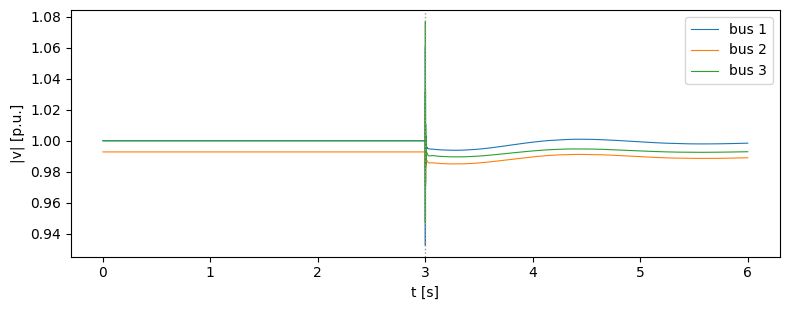
res.voltage maps each bus to its complex voltage trajectory. The line opening at t = 3 s and the electromagnetic transient it excites are both visible:

fig, ax = plt.subplots(figsize=(8, 3.2))
for bus in res.buses():
    ax.plot(res.t, res.voltage_magnitude(bus), lw=0.8, label=f"bus {bus}")
ax.axvline(3.0, color="0.6", ls=":", lw=1)
ax.set_xlabel("t [s]")
ax.set_ylabel("|v| [p.u.]")
ax.legend()
fig.tight_layout()

Every device keeps its own differential states, listed per unit in res.devices:

for dev in res.devices:
    print(f"{dev.unit} at bus {dev.bus}: {', '.join(dev.states)}")

SG1 at bus 1: delta, omega, psv, pm, Efd, Rf, Vr, e_dprim, e_qprim, psid, psiq, psid2, psiq2
GFMI2 at bus 3: Vfd_ext, Vfq_ext, ifd_ext, ifq_ext, itd_ext, itq_ext, Pc_tilde, delta_c, Qc_tilde, xi_d, xi_q, gamma_d, gamma_q

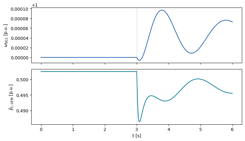
The machine speed and the converter’s filtered active power tell the electromechanical story of the event: the converter picks up the power the lost line no longer carries, and the machine settles at a slightly different angle.

sg1 = next(d for d in res.devices if d.unit == "SG1")
gfm = next(d for d in res.devices if d.unit == "GFMI2")

fig, axes = plt.subplots(2, 1, figsize=(8, 4.6), sharex=True)
axes[0].plot(res.t, sg1.states["omega"], color="#215CAF")
axes[0].set_ylabel(r"$\omega_{\mathrm{SG1}}$ [p.u.]")
axes[1].plot(res.t, gfm.states["Pc_tilde"], color="#007894")
axes[1].set_ylabel(r"$\tilde p_{c,\mathrm{GFM}}$ [p.u.]")
axes[1].set_xlabel("t [s]")
for ax in axes:
    ax.axvline(3.0, color="0.6", ls=":", lw=1)
fig.tight_layout()

From here, each of the remaining notebooks picks out one aspect of the simulator: scheduled disturbances, the hybrid EMT/RMS network, small-signal analysis and parametric sensitivities. The user guide describes the system files, and the model library documents every device class.