Converters

A converter is composed in exactly the same manner as a machine: the converter class implements the power path (the voltage-source converter behind its LCL output filter), and the control blocks are pluggable strategies on five axes, the output filter, the angle source, the voltage control, the inner control and the PLL (see Converter control strategies). Three converter classes ship, differing in how they synchronize and in which strategies they plug in by default. GridForming sets its own frequency and voltage from an active-power droop. GridSupporting rides on a PLL and adds the droop on the PLL frequency, keeping the full voltage-mode cascade. GridFollowing also rides on a PLL but replaces that cascade by a current-injecting chain of power-PI and current-PI controllers.

Class	Description
Inverter	Base class of all converter models: composition of the pluggable filter, angle-source, voltage-control, inner-control and PLL strategies with the power measurement filter and the network coupling.
GridFollowing	Grid-following converter (the literature-standard current-injecting chain, as in PowerSimulationsDynamics.jl and its PSCAD benchmarks): the converter frame IS the PLL frame, PI controllers on the filtered active and reactive power produce dq current commands, and a current-mode inner loop tracks them on the LCL filter.
GridSupporting	Grid-supporting converter (the grid-supporting voltage source of the Rocabert et al. taxonomy): the converter frame rides on a synchronous-reference-frame PLL, with the active-power droop added on the PLL frequency and the full voltage-mode cascade behind it, so the converter supports the grid it synchronizes to (model of https://doi.org/10.1109/TPWRS.2021.3061434; named GridFollowing before v1.1, when that name moved to the current-injecting PI chain of GridFollowing).
GridForming	Grid-forming converter: the droop angle source sets the converter frequency from the filtered active power, so the converter behaves as a voltage source behind its LCL filter (model of https://doi.org/10.1109/TPWRS.2021.3061434).

In the voltage-mode chain of the grid-forming and grid-supporting converters, the filter strategy carries the plant states \(v_f, i_f, i_t\); the angle source sets the converter frequency \(\omega_c\) and angle \(\delta_c\) (from the active-power droop for a grid-forming unit, from the PLL for a grid-supporting unit); the voltage controller turns the reactive-power error into the voltage command \(V_{cd}\); the inner controller closes the cascaded voltage and current loops and produces the switching voltage \(v_{sw}^{*}\); and the PLL tracks the filter-voltage phasor:

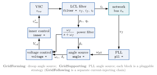
How a grid-forming or grid-supporting converter is composed: the converter class implements the power path; filter, angle source, voltage control, inner control and PLL are pluggable strategies selected by keyword on the converter line.

In the current-injecting chain of the grid-following converter, the converter frame is the PLL frame itself. PI controllers on the filtered active and reactive power occupy the angle and voltage slots and produce the dq current commands, and a current-mode inner loop tracks them on the same LCL filter:

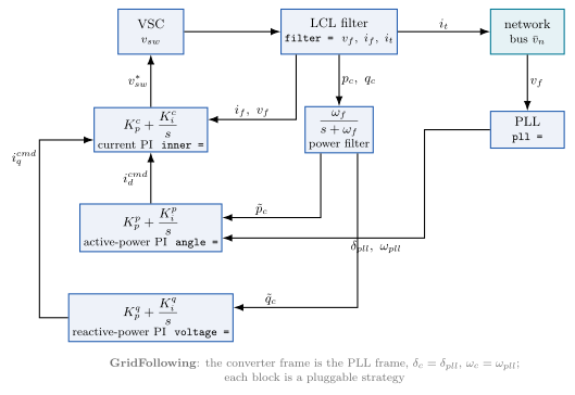
How a grid-following converter is composed: the same power path, with the power-PI outers and the current-mode inner loop in the strategy slots and the PLL fixing the converter frame.

Converter base class

The parent class of all converter models. It introduces the shared parameters and the initialization procedure, and wires the five pluggable control blocks.

class hermess.devices.inverter.Inverter(filter=None, pll=None, angle=None, voltage=None, inner=None)

Base class of all converter models: composition of the pluggable

filter, angle-source, voltage-control, inner-control and PLL strategies with the power measurement filter and the network coupling.

The strategy blocks and their equations are documented in their own classes (hermess.devices.inverter_filter, inverter_angle, inverter_voltage, inverter_inner, inverter_pll); this base owns the instantaneous terminal powers and their measurement filter,

\[\begin{split}p_c &= v_{fd} i_{td} + v_{fq} i_{tq}, \qquad q_c = -v_{fd} i_{tq} + v_{fq} i_{td} \\ \dot{\tilde{p}}_c &= \omega_f \, (p_c - \tilde{p}_c), \qquad \dot{\tilde{q}}_c = \omega_f \, (q_c - \tilde{q}_c),\end{split}\]

and the injection of the grid-side current \(i_t\) (rotated by the converter angle \(\delta_c\) and rescaled by \(S_n/S_b\)) into the network current balance. All quantities are in per unit on the device base \(S_n\), with \(\omega_b = 2\pi f_n\).

Symbols (owned by the base; strategy parameters are documented in the strategy classes):

Code	Symbol	Meaning	Default
Sn	\(S_n\)	converter MVA rating (device base) [MVA]	100
Vn	\(V_n\)	rated voltage [kV]	-
fn	\(f_n\)	rated frequency [Hz]	50
omega_f	\(\omega_f\)	power measurement filter corner frequency [rad/s]	2pi5
omega_f_q	\(\omega_f^{q}\)	Q-side filter corner frequency [rad/s] (default: follows omega_f)	NaN
Pc_tilde	\(\tilde{p}_c\)	filtered active power (state) [p.u.]
Qc_tilde	\(\tilde{q}_c\)	filtered reactive power (state) [p.u.]
Pc / Qc	\(p_c, q_c\)	unfiltered terminal powers (published expressions)
Pref	\(p_c^{*}\)	active-power setpoint (set by the initialization)
Qref	\(q_c^{*}\)	reactive-power setpoint (set by the initialization)
Vref	\(v_c^{*}\)	voltage setpoint (set by the initialization)

current_command(dae)

Outer current commands (Idc_cmd, Iqc_cmd), host-mediated: published by the power-PI outer strategies (PLLPowerPI / QPowerPI) and read by the current-mode inner control. None when the selected outers publish a voltage command instead.

Parameters:

dae (Dae)

current_ref(dae)

Inner current references (ifd_ref, ifq_ref), host-mediated: published by the inner strategy and read back by its own current loop. This accessor is the interception seam for a future current limiter, which would resolve it to a saturated var_sym algebraic (i* = sat(iref)).

Parameters:

dae (Dae)

fgcall(dae)

Orchestrate the pluggable converter strategies into the DAE residual.

The host owns only the cross-cutting glue: the reference-frame frequency, the Park transforms into the converter frame, the power measurement, and the power-measurement filters. Everything else is delegated, in signal-flow order: PLL -> angle source (omega_c, delta_c) -> voltage control (Vcd) -> inner control (Vsw) -> filter (LCL). Each strategy reads host params/states by attribute and writes its own equations; the host threads the symbolic intermediates (omega_c, Vcd, Vsw) between them.

Return type:

None

Parameters:

dae (Dae)

finit_anchor_residuals(dae)

Extra steady-state anchor residuals (each an n-vector that must equal 0) a device declares to keep its initialization Newton system square.

The joint init pins each device’s state ODEs (f = 0) plus two quantities through the bus-current balance (g[vre]/g[vim]), so a square system requires n_setpoints == 2 (the SG: Pref + Vref). A device with more setpoints returns n_setpoints - 2 anchor residuals to balance them. Empty by default.

Example: the inverter has 3 setpoints (Pref/Qref/Vref) but the bus equations pin only 2; it returns one anchor (Qref = Qc) here.

Return type:

list

Parameters:

dae (Dae)

pll_frequency(dae)

Synchronizing frequency from the PLL, host-mediated: the PLL’s omega_pll when a PLL strategy is present, else nominal omega_net (no PLL => no estimate). Consumers read this accessor and never reference the PLL strategy directly.

Return type:

SX

Parameters:

dae (Dae)

switching_voltage(dae)

Switching voltage (Vswd, Vswq) in the network frame, host-mediated: published by the inner strategy and read by the filter. A symbolic intermediate, not a DAE variable.

Parameters:

dae (Dae)

static to_external(d_int, q_int, delta)

Park-rotate (d, q) from the converter (internal) frame back to the network (external) frame defined by angle delta.

static to_internal(d_ext, q_ext, delta)

Park-rotate (d, q) from the network (external) frame into the converter (internal) frame defined by angle delta.

var_sym(dae, name)

Resolve a registered variable name to its symbol wherever it lives: dae.y for a device-private algebraic, dae.x for a differential state. Lets the converter equations read a coupling quantity (a filter state, the frame angle, …) regardless of whether a given realization made it a state or an algebraic (dynamic LCL states vs quasi-static LCL_static algebraics).

Return type:

SX

Parameters:

• dae (Dae)

• name (str)

voltage_command(dae)

Voltage-magnitude reference Vcd, host-mediated: published by the voltage strategy’s fgcall and read by the inner controller. A symbolic intermediate, not a DAE variable.

Return type:

SX

Parameters:

dae (Dae)

Grid-forming converter

A grid-forming converter, which sets its own frequency and voltage. The small-signal behavior in low-inertia systems follows [2].

class hermess.devices.inverter.GridForming(filter=None, angle=None, voltage=None, inner=None, pll=None)

Grid-forming converter: the droop angle source sets the converter

frequency from the filtered active power, so the converter behaves as a voltage source behind its LCL filter (model of https://doi.org/10.1109/TPWRS.2021.3061434).

Selected in a system file by the class name in the first column:

GridForming, idx = "GFM1", bus = "3", Sn = 100, Kp = 0.01, Kq = 0.1, ...

Model. The equations below are the assembled set for the default strategy combination (dynamic LCL filter, Droop angle, QVDroop voltage control, Cascaded inner control); each block’s own class documents its variants, and the parameter symbols are listed in the strategy classes and Inverter.

Converter Voltage Dynamics

\[\begin{split}\dot{v}_{fd_{ext}} &= \frac{\omega_{b}}{c_{f}}(i_{fd_{ext}} - i_{td_{ext}}) + \omega_{net}\omega_{b}v_{fq_{ext}} \\ \dot{v}_{fq_{ext}} &= \frac{\omega_{b}}{c_{f}}(i_{fq_{ext}} - i_{tq_{ext}}) - \omega_{net}\omega_{b}v_{fd_{ext}}\end{split}\]

Converter Current Dynamics

\[\begin{split}\dot{i}_{fd_{ext}} &= \frac{\omega_{b}}{l_{f}}(v_{swd} - v_{fd_{ext}}) - \frac{\omega_{b}r_{f}}{l_{f}}i_{fd_{ext}} + \omega_{net}\omega_{b}i_{fq_{ext}} \\ \dot{i}_{fq_{ext}} &= \frac{\omega_{b}}{l_{f}}(v_{swq} - v_{fq_{ext}}) - \frac{\omega_{b}r_{f}}{l_{f}}i_{fq_{ext}} - \omega_{net}\omega_{b}i_{fd_{ext}}\end{split}\]

Grid-Side Current Dynamics

\[\begin{split}\dot{i}_{td_{ext}} &= \frac{\omega_b}{l_t}(v_{fd_{ext}} - v_{n_{re}}) - \frac{\omega_b r_t}{l_t}i_{td_{ext}} + \omega_{net} \omega_b i_{tq_{ext}} \\ \dot{i}_{tq_{ext}} &= \frac{\omega_b}{l_t}(v_{fq_{ext}} - v_{n_{im}}) - \frac{\omega_b r_t}{l_t}i_{tq_{ext}} - \omega_{net} \omega_b i_{td_{ext}}\end{split}\]

Power and Frequency Dynamics

\[\begin{split}\dot{\tilde{p}}_{c} &= \omega_{f}(p_{c} - \tilde{p}_{c}) \\ \delta\dot{\theta}_{c} &= \omega_{b}\delta\omega_{c} \\ \dot{\tilde{q}}_{c} &= \omega_{f}(q_{c} - \tilde{q}_{c})\end{split}\]

Control Dynamics

\[\begin{split}\dot{\xi}_{d} &= v_{fd^{*}} - v_{fd_{int}} \\ \dot{\xi}_{q} &= v_{fq^{*}} - v_{fq_{int}} \\ \dot{\gamma}_{d} &= i_{fd^{*}} - i_{fd_{int}} \\ \dot{\gamma}_{q} &= i_{fq^{*}} - i_{fq_{int}}\end{split}\]

Grid-supporting converter

A grid-supporting converter, which synchronizes to the grid through a PLL and adds the active-power droop on the PLL frequency, keeping the full voltage-mode cascade [2]. The class was named GridFollowing before v1.1, when that name moved to the current-injecting chain below.

class hermess.devices.inverter.GridSupporting(filter=None, angle=None, voltage=None, inner=None, pll=None)

Grid-supporting converter (the grid-supporting voltage source of the

Rocabert et al. taxonomy): the converter frame rides on a synchronous-reference-frame PLL, with the active-power droop added on the PLL frequency and the full voltage-mode cascade behind it, so the converter supports the grid it synchronizes to (model of https://doi.org/10.1109/TPWRS.2021.3061434; named GridFollowing before v1.1, when that name moved to the current-injecting PI chain of GridFollowing).

Selected in a system file by the class name in the first column:

GridSupporting, idx = "GS1", bus = "5", Sn = 100, Kp = 0.01, ...

Model. The equations below are the assembled set for the default strategy combination (dynamic LCL filter, PLL angle source, SRF_PLL); each block’s own class documents its variants, and the parameter symbols are listed in the strategy classes and Inverter.

Converter Voltage Dynamics

\[\begin{split}\dot{v}_{fd_{ext}} &= \frac{\omega_{b}}{c_{f}}(i_{fd_{ext}} - i_{td_{ext}}) + \omega_{net}\omega_{b}v_{fq_{ext}} \\ \dot{v}_{fq_{ext}} &= \frac{\omega_{b}}{c_{f}}(i_{fq_{ext}} - i_{tq_{ext}}) - \omega_{net}\omega_{b}v_{fd_{ext}}\end{split}\]

Converter Current Dynamics

\[\begin{split}\dot{i}_{fd_{ext}} &= \frac{\omega_{b}}{l_{f}}(v_{swd} - v_{fd_{ext}}) - \frac{\omega_{b}r_{f}}{l_{f}}i_{fd_{ext}} + \omega_{net}\omega_{b}i_{fq_{ext}} \\ \dot{i}_{fq_{ext}} &= \frac{\omega_{b}}{l_{f}}(v_{swq} - v_{fq_{ext}}) - \frac{\omega_{b}r_{f}}{l_{f}}i_{fq_{ext}} - \omega_{net}\omega_{b}i_{fd_{ext}}\end{split}\]

Grid-Side Current Dynamics

\[\begin{split}\dot{i}_{td_{ext}} &= \frac{\omega_b}{l_t}(v_{fd_{ext}} - v_{n_{re}}) - \frac{\omega_b r_t}{l_t}i_{td_{ext}} + \omega_{net} \omega_b i_{tq_{ext}} \\ \dot{i}_{tq_{ext}} &= \frac{\omega_b}{l_t}(v_{fq_{ext}} - v_{n_{im}}) - \frac{\omega_b r_t}{l_t}i_{tq_{ext}} - \omega_{net} \omega_b i_{td_{ext}}\end{split}\]

Phase-Locked Loop (PLL) Dynamics

\[\begin{split}\dot{\epsilon} &= v_{fq_{pll}} \\ \delta\dot{\theta}_{pll} &= \omega_{b}\delta\omega_{pll}\end{split}\]

Power and Frequency Dynamics

\[\begin{split}\dot{\tilde{p}}_{c} &= \omega_{f}(p_{c} - \tilde{p}_{c}) \\ \delta\dot{\theta}_{c} &= \omega_{b}\delta\omega_{c} \\ \dot{\tilde{q}}_{c} &= \omega_{f}(q_{c} - \tilde{q}_{c})\end{split}\]

Control Dynamics

\[\begin{split}\dot{\xi}_{d} &= v_{fd^{*}} - v_{fd_{int}} \\ \dot{\xi}_{q} &= v_{fq^{*}} - v_{fq_{int}} \\ \dot{\gamma}_{d} &= i_{fd^{*}} - i_{fd_{int}} \\ \dot{\gamma}_{q} &= i_{fq^{*}} - i_{fq_{int}}\end{split}\]

Grid-following converter

A grid-following converter in the literature-standard current-injecting form, matching the PowerSimulationsDynamics.jl reference model and its PSCAD benchmarks: the frame rides on the PLL, power-PI outers produce the current commands and a current-mode inner loop tracks them.

class hermess.devices.inverter.GridFollowing(filter=None, angle=None, voltage=None, inner=None, pll=None)

Grid-following converter (the literature-standard current-injecting

chain, as in PowerSimulationsDynamics.jl and its PSCAD benchmarks): the converter frame IS the PLL frame, PI controllers on the filtered active and reactive power produce dq current commands, and a current-mode inner loop tracks them on the LCL filter. Introduced in v1.1; the PLL-anchored droop chain that carried this name before is GridSupporting.

Selected in a system file by the class name in the first column:

GridFollowing, idx = "GFL1", bus = "5", Sn = 100, Kpp = 2, Kip = 30, ...

Model. The default strategy combination is LCL filter, PLLPowerPI angle source (frame = PLL, active-power PI), QPowerPI voltage slot (reactive-power PI), CurrentPI inner control and ReducedPLL; each block’s own class documents its equations, and the parameter symbols are listed in the strategy classes and Inverter. The chain, in signal-flow order:

\[\begin{split}0 &= -\delta_c + \delta_{pll} \\ i_{d}^{cmd} &= K_p^{p} ( p_c^{*} - \tilde{p}_c ) + K_i^{p} \sigma_p \\ i_{q}^{cmd} &= -\left[ K_p^{q} ( q_c^{*} - \tilde{q}_c ) + K_i^{q} \sigma_q \right] \\ v_{swdq} &= K_p^c ( i_{dq}^{cmd} - i_{fdq} ) + K_i^c \gamma_{dq} \mp \omega_c l_f i_{fqd} + K_{ff}^c v_{fdq}\end{split}\]

with the six LCL filter states as in GridForming and the PLL as documented in its strategy class.

References

[2] (1,2)

U. Markovic, O. Stanojev, P. Aristidou, E. Vrettos, D. Callaway, and G. Hug, Understanding Small-Signal Stability of Low-Inertia Systems, IEEE Transactions on Power Systems, vol. 36, no. 5, pp. 3997-4017, Sep. 2021, doi: 10.1109/TPWRS.2021.3061434.