Graphical interface

HERMESS ships an optional desktop GUI for interactive work: pick a system, adjust the simulation settings, run, and inspect the trajectories, the small-signal modes and the initial power flow without writing a script. It is aimed at exploratory research use and at teaching; batch work and paper pipelines are better served by the Python API (Running simulations).

Installation and launch

The GUI dependencies (PySide6, pyqtgraph) are an optional extra, so the core package stays lightweight:

pip install -e ".[gui]"     # or:  uv sync --extra gui

Launch it with either of:

hermess-gui
python -m hermess.gui

The window layout, the opened folders, the selected system and the simulation options persist across sessions.

Layout

The window follows the classic desktop tool arrangement. The Systems panel on the left lists the systems shipped with the package and any folders you open, with an inspector showing the selected system’s devices, lines, bus initialization and disturbances, parsed read-only from its text files, plus the raw files themselves. The central area holds four viewer tabs, described below. The Log panel at the bottom receives the simulation log, the initial power flow and the modal report. The toolbar carries Run (F5), Stop, the options dialog, the CSV export and a selector over the finished runs of the session (the last ten are kept).

Simulations execute in a separate worker process, so the interface stays responsive during long runs and Stop cancels cleanly. Progress is reported in the status bar; with disturbances and incl_lim off, cancellation takes effect between disturbance intervals.

Running a simulation

Select a system and press Run. The settings behind hermess.simulate() are edited in the options dialog (Simulation → Options), which exposes the fields of Config: end time, time step, integration scheme and its options, reference-frame mode, dynamic or quasi-static lines, limiters, and the small-signal analysis switch. Only values you change are carried as overrides; everything else follows the shipped defaults, overlaid with the selected system’s own sim_settings.txt when it has one (the dialog names those defaults), exactly as hermess.simulate() applies them.

To simulate systems of your own, use Open folder… and point it either at a single system folder (containing sim_param.txt and optionally sim_dist.txt) or at a directory holding several such folders. Externally edited files are picked up with Reload; systems can also be built and modified graphically (see Building systems).

Pre-flight checks

Run first validates the system and the options together, so common mistakes surface as one dialog instead of a failed run. Hard errors block the start: a network that is not fully connected (with the detached bus groups named), an ODE-only integration scheme (cvodes, rk) applied to a model with algebraic variables, a single reference frame pointing at a device that does not exist in the file, more than one injector on a bus, duplicate unit identifiers, or a time step that is non-positive or larger than the end time. Questionable but runnable settings, such as a quasi-static inverter filter on a dynamic network or a very large number of output steps, are listed as warnings and ask for confirmation.

When the small-signal analysis is enabled, the run additionally pauses at the initialized operating point if unstable modes are found: a dialog lists them (eigenvalue, frequency, damping ratio and dominant states) and asks whether to continue or stop, before any time is spent on an integration that will likely diverge. Stable operating points are noted in the log and the run proceeds without interruption.

Viewer tabs

Topology

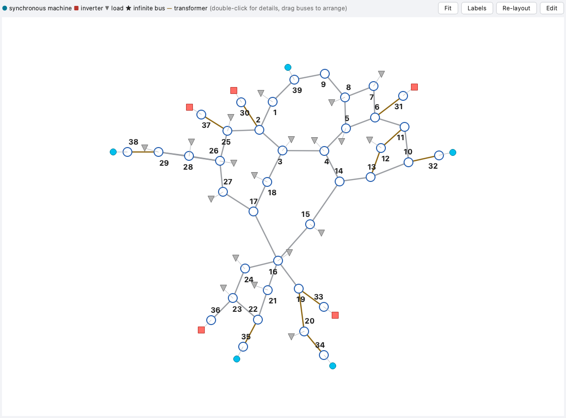
A one-line diagram of the selected system, available before any run. Buses are laid out automatically and can be dragged; devices appear as glyphs attached to their buses (circle for a synchronous machine, square for an inverter, triangle for a load), and transformer branches are drawn in bronze. After a run of the same system, every bus is annotated with its initialized voltage magnitude and angle.

Double-clicking any component opens a detail pop-up: for a device, a short model description with the matching control schematics (the same block diagrams as in Model library) and the parameters from the system file; for a bus, its initialization, the connected branches and devices, and the initialized voltage of the shown run; for a line, its parameters and the pi-section schematic.

Building systems

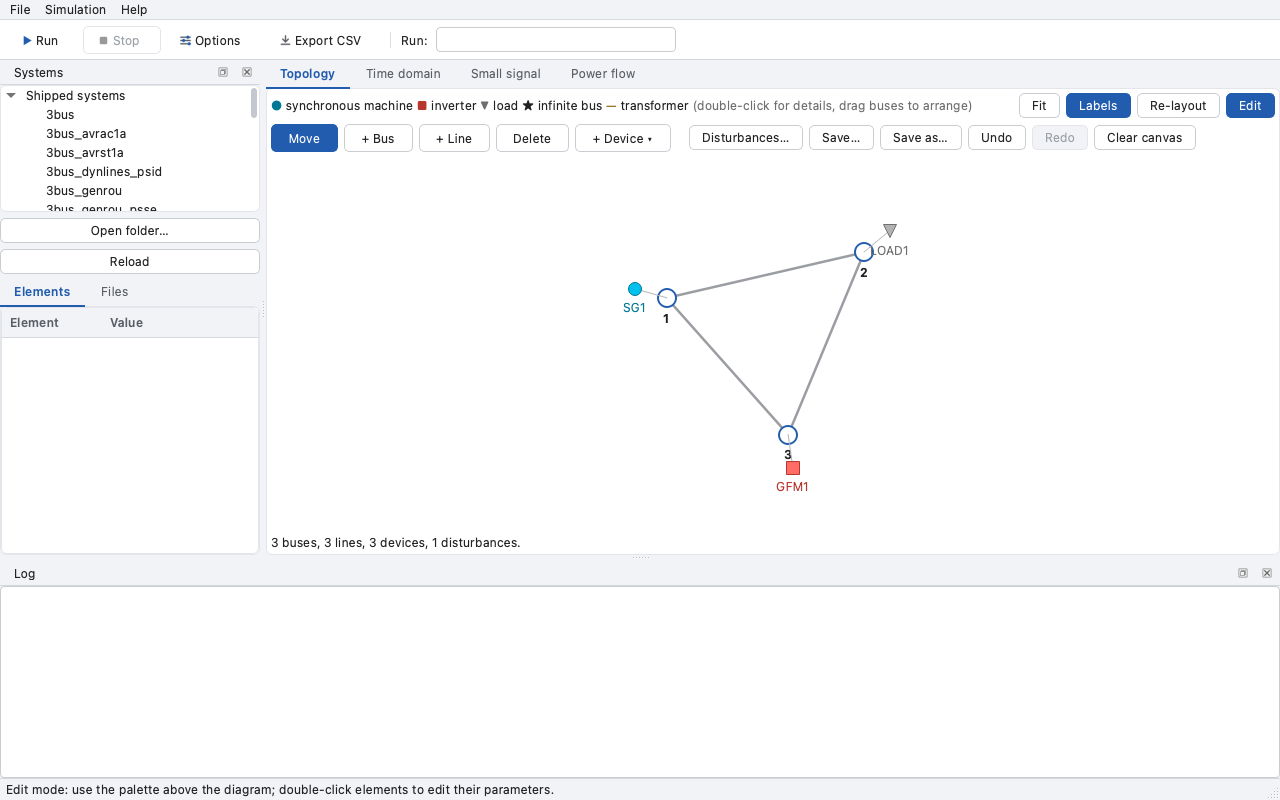
The Edit toggle above the diagram turns the topology view into a builder. A palette provides the tools: + Bus places a bus where you click (the first one becomes the slack), + Line connects two clicked buses, + Device offers every available model, shipped or registered through hermess.register(), and attaches the chosen one to a clicked bus, Delete removes what you click, and Disturbances… edits the event sequence, with every field labeled by the core’s own explanation and units, required fields enforced, and the equivalent sim_dist.txt line shown for the selected event type. Double-clicking an element in edit mode, lines included, opens its parameter form instead of the detail pop-up. File > New system starts from a blank canvas, Clear canvas empties the current one after a confirmation (and stays undoable), and entering edit mode on a selected system edits a copy of it. The usual undo/redo shortcuts work, and Escape abandons a half-drawn line.

The parameter forms are generated from the model classes themselves: every parameter appears with its default greyed in and its meaning as a tooltip, and the control strategies (AVR, governor, PSS, shaft; filter, angle, voltage, inner control, PLL) are chosen from dropdowns that regenerate the form and name what the model default resolves to. The unit identifier shows the name that will be generated when left empty. After placing a line or a device, or deleting something, the active tool falls back to Move so stray clicks stay inert, and the mouse cursor indicates the active tool. Fields left empty use the model defaults and are not written to the file, so generated files stay as terse as hand-written ones.

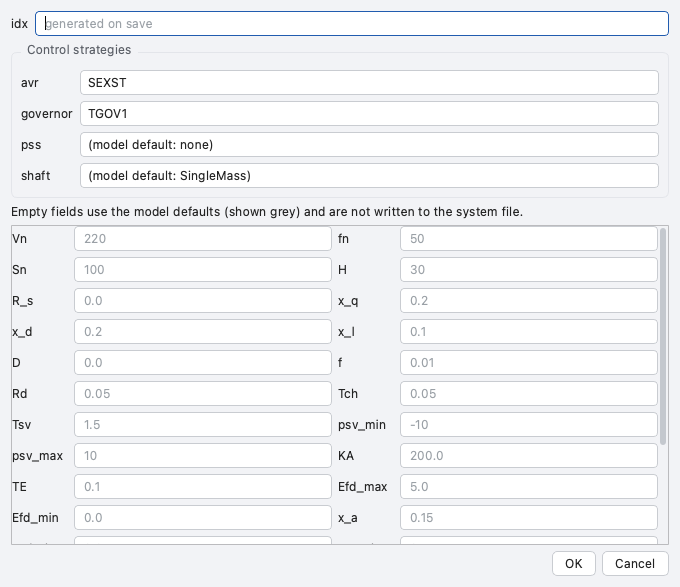
While editing, the status line below the canvas shows the live validation of the pre-flight checks (connectivity, slack bus, solver compatibility, shunt susceptance under dynamic lines, one injector per bus, unique unit identifiers), and every change is undoable. Saving writes an ordinary system folder (sim_param.txt + sim_dist.txt) to a location of your choice, never into the installed package; the saved system appears in the browser and runs, exports and versions like any other. Re-saving a hand-written system rewrites its files without preserving comments, so editing an imported system defaults to Save as. When a saved network’s lines carry no charging (so it cannot run with dynamic lines), the GUI offers once to write a sim_settings.txt with line_dyn = false next to it, making the system run out of the box everywhere; declining is remembered and nothing is ever reclassified silently.

No saving is needed while composing. Because a run executes from the files on disk (the same ones scripts and the CLI use, so every run stays reproducible), Run asks for a save location the first time; from then on, running an edited system saves it automatically, and the Save… and Save as… buttons in the palette (or the usual shortcuts) work at any time. Save as… forks the current state into a new folder, suggested next to the original, which is the way to keep a variant for comparison with a system built earlier. Every document saves only into its own folder, so systems built in parallel never overwrite each other; picking a folder that already holds a different system in Save as asks before replacing it. While a document is being edited, the systems browser is deselected and its inspector emptied, so the left column never shows a stale system; leaving edit mode asks about unsaved changes and restores the previously shown system.

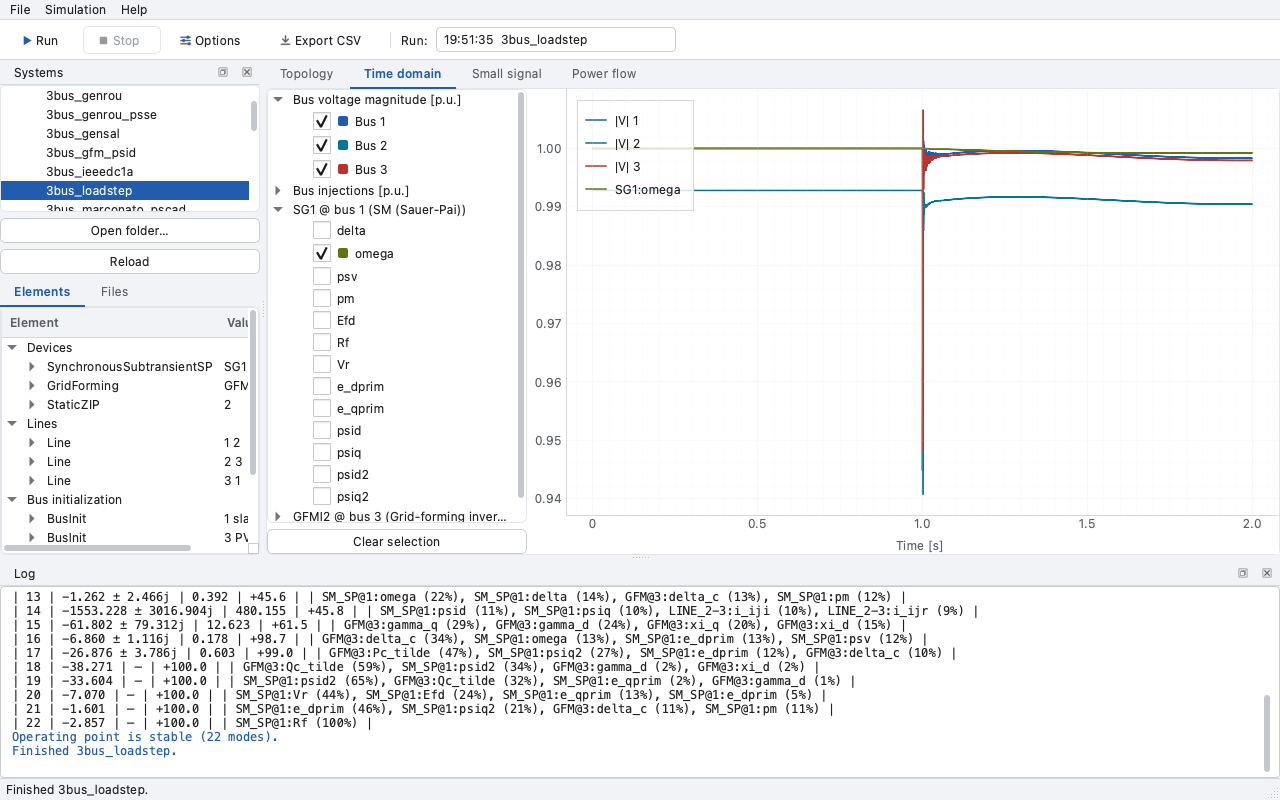
Time domain

The trajectories of the shown run: bus voltage magnitudes, bus injections, every device’s differential states, and the device-level algebraic signals, marked “(algebraic)” in the tree. The latter cover the private algebraic variables (e.g. the quasi-static filter quantities) and the outputs the models expose symbolically, such as a grid-forming converter’s frequency omega_c, evaluated over the stored trajectories. Everything is selected in the tree and overlaid in one interactive plot (zoom, pan, automatic downsampling for long records); the panes are resized by dragging the divider between them.

Small signal

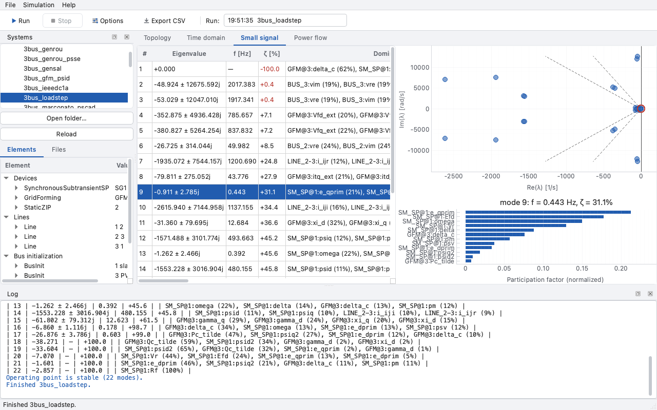
The modal analysis at the operating point, when small_signal_analysis is enabled in the options. The table lists the physical modes (conjugate pairs collapsed) with frequency and damping ratio, sorted most critical first; the map shows the eigenvalues with constant-damping guide rays. Selecting a mode, in the table or by clicking an eigenvalue, highlights it and shows its normalized participation factors as a bar chart.

Power flow

The initial power flow of the shown run as sortable bus and branch tables, the same data power_flow_tables() returns.

Exporting results

File → Export CSV… writes the signals currently checked in the time-domain tree as a plot-ready CSV (a t column plus one named column per signal, with a header row), together with a .provenance.txt sidecar recording the system, the settings, the package version and the date. This is the intended bridge into a paper’s data/ directory. File → Export figure… saves the current tab as a PNG for quick sharing; publication figures should be built from the exported data instead.