Parametric sensitivities

With parametric=True the equations are assembled with every device parameter as a CasADi symbol. The run itself is unchanged, but the returned model keeps the parametric expressions, so a functional of the trajectory can be differentiated with respect to all parameters at the cost of one reverse-mode sweep, independent of how many parameters there are.

This notebook builds the parametric 3-bus model, perturbs the machine speed off its equilibrium, defines the energy of the speed deviation as the functional, and computes its gradient with respect to every device parameter at once. Two entries, the machine inertia and the converter droop, are then checked against finite differences.

The run itself is configured for smoothness, which adjoint differentiation rewards: no disturbance, no state limiters, and a fixed nominal reference frequency.

import casadi as ca
import numpy as np

import hermess

dae = hermess.simulate(
    "3bus", T_end=0.5, ts=5e-3, line_dyn=False, parametric=True,
    skip_disturance=True, incl_lim=False, omega_mode="nom",
    log_level="ERROR",
)
model = dae.parametric_model
print(f"{model.p.numel()} symbolic parameters")

Simulation: 100%|██████████| 100.0/100% [00:00<00:00]

61 symbolic parameters

model.dae_dict() packages the parametric model for casadi.integrator, with the parameter vector appended to the input. Integrate 0.5 s after kicking the machine speed by 2e-3 p.u., and define \(J = \sum_k (\omega_k - 1)^2\) over the trajectory:

grid = np.arange(0.01, 0.5, 0.01)
I = ca.integrator("I", "idas", model.dae_dict(), 0.0, grid,
                  {"reltol": 1e-10, "abstol": 1e-12})

machine = dae.device_list[0]
x0 = np.array(dae.xinit)
x0[machine.omega] += 2e-3

p = ca.MX.sym("p", model.p.numel())
sol = I(x0=x0, z0=dae.yinit, p=ca.vertcat(ca.DM.ones(dae.nx), p))
J = ca.sumsqr(sol["xf"][int(machine.omega[0]), :] - 1.0)

J_of_p = ca.Function("J", [p], [J])
dJ_of_p = ca.Function("dJ", [p], [ca.gradient(J, p)])

gradient = np.array(dJ_of_p(model.p_val)).ravel()
print(f"J at nominal parameters: {float(J_of_p(model.p_val)):.3e}")

J at nominal parameters: 9.587e-05

model.slice_of locates one parameter of one device in the stacked vector. Check the machine inertia and the converter droop against central finite differences of the same functional:

for device, name in (("SG1", "H"), ("GFMI2", "Kp")):
    idx = model.slice_of(device, name).start
    h = 1e-5 * max(1.0, abs(model.p_val[idx]))
    p_plus, p_minus = model.p_val.copy(), model.p_val.copy()
    p_plus[idx] += h
    p_minus[idx] -= h
    fd = (float(J_of_p(p_plus)) - float(J_of_p(p_minus))) / (2 * h)
    print(f"dJ/d{name} of {device}:  reverse-mode {gradient[idx]: .6e}"
          f"   finite diff. {fd: .6e}")

dJ/dH of SG1:  reverse-mode  8.609925e-06   finite diff.  8.609744e-06
dJ/dKp of GFMI2:  reverse-mode  1.851819e-03   finite diff.  1.851818e-03

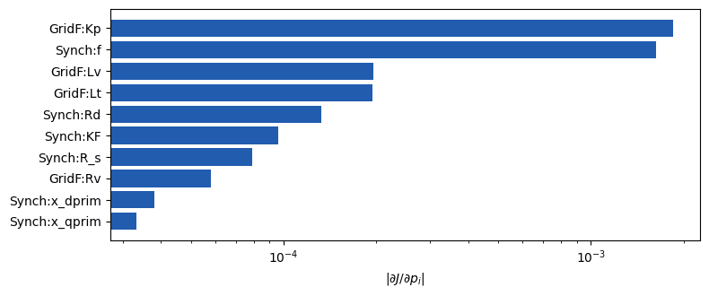
The gradient covers every parameter of every device in the system, so the same sweep also ranks which parameters the functional is sensitive to at all. The speed-deviation energy responds to the machine parameters and to the converter’s droop and filter constants, and barely to anything else:

import matplotlib.pyplot as plt

labels = [f"{type(e.device).__name__.split('_')[0][:5]}:{e.name}"
          for e in model.entries]
order = np.argsort(np.abs(gradient))[::-1][:10]

fig, ax = plt.subplots(figsize=(8, 3.4))
ax.barh(range(len(order))[::-1], np.abs(gradient[order]), color="#215CAF")
ax.set_yticks(range(len(order))[::-1])
ax.set_yticklabels([labels[i] for i in order])
ax.set_xscale("log")
ax.set_xlabel(r"$|\partial J / \partial p_i|$")
fig.tight_layout()

Setpoints and line parameters stay numeric (the initialization overwrites the former and the admittance matrices absorb the latter), and the operating point itself is evaluated at the nominal values; the sensitivities page of the user guide states the exact scope.